
| 일 | 월 | 화 | 수 | 목 | 금 | 토 |
|---|---|---|---|---|---|---|
| 1 | 2 | 3 | 4 | |||
| 5 | 6 | 7 | 8 | 9 | 10 | 11 |
| 12 | 13 | 14 | 15 | 16 | 17 | 18 |
| 19 | 20 | 21 | 22 | 23 | 24 | 25 |
| 26 | 27 | 28 | 29 | 30 | 31 |
- 카카오
- 데이터사이언스 스쿨
- 재귀함수
- numpy
- TensorFlow
- 제로베이스 데이터사이언스
- Set
- 추천시스템
- 데이터사이언티스트
- 머신러닝
- 아이펠
- AIFFEL
- 사이킷런
- 클래스
- 파이썬코딩도장
- 후기
- AI
- 딕셔너리
- NLP
- 코딩도장
- 자연어처리
- 데이터분석
- 스크랩
- 파이썬
- Python
- 딥러닝
- 제어문
- 함수
- 기사
- 속성
- Today
- Total
뮤트 개발일지
AIFFEL 아이펠 19일차 본문
딥러닝 들여다보기
신경망 구성
MNIST 이미지 분류기
# Tensorflow 기반 분류 모델 예시 코드

import tensorflow as tf
from tensorflow import keras
import numpy as np
import matplotlib.pyplot as plt

# MNIST 데이터를 로드. 다운로드하지 않았다면 다운로드까지 자동으로 진행됩니다.
mnist = keras.datasets.mnist
(x_train, y_train), (x_test, y_test) = mnist.load_data()

# 모델에 맞게 데이터 가공
x_train_norm, x_test_norm = x_train / 255.0, x_test / 255.0
x_train_reshaped = x_train_norm.reshape(-1, x_train_norm.shape[1]*x_train_norm.shape[2])
x_test_reshaped = x_test_norm.reshape(-1, x_test_norm.shape[1]*x_test_norm.shape[2])

# 딥러닝 모델 구성 - 2 Layer Perceptron
model=keras.models.Sequential()
model.add(keras.layers.Dense(50, activation='sigmoid', input_shape=(784,)))  # 입력층 d=784, 은닉층 레이어 H=50
model.add(keras.layers.Dense(10, activation='softmax'))   # 출력층 레이어 K=10
model.summary()

# 모델 구성과 학습
model.compile(optimizer='adam',
             loss='sparse_categorical_crossentropy',
             metrics=['accuracy'])
model.fit(x_train_reshaped, y_train, epochs=10)

# 모델 테스트 결과
test_loss, test_accuracy = model.evaluate(x_test_reshaped,y_test, verbose=2)
print("test_loss: {} ".format(test_loss))
print("test_accuracy: {}".format(test_accuracy))
이미지 설명)
은닉층에 H개의 노드가, 출력충에 K개의 노드가 있다.
위의 코드에서는 h=50, k=10, d=784로 정의되어 있다.
보통 입력층과 출력층 사이에 있는 층은 모두 은닉층이라고 부른다.
은닉층이 많아질수록 인공신경망이 deep해졌다고 말한다.
Parameters/Weights
입력층-은닉층, 은닉층-출력층 사이에는 행렬Matrix이 존재한다. 예로 입력값이 100개, 은닉 노드가 20개면 입력층-은닉층 사이에는 100*20의 형태를 가진 행렬이 존재한다. 또한 10개의 클래스를 맞추는 문제를 풀기 위해 출력층이 10개의 노드를 가진다면 은닉층-출력층 사이에는 20*10의 형태를 가진 행렬이 존재한다. 이 행렬들을 parameter 혹은 weight라고 부른다.
이 때, 인접한 레이어 사이에는 다음과 같은 관계가 성립한다.
y = W * X + b
활성화 함수 Activation Functions
1. 시그모이드 Sigmoid

2. Tahn

3. ReLU

읽을 거리...
딥러닝에서 사용하는 활성화함수
An Ed edition
reniew.github.io
https://pozalabs.github.io/Activation_Function/
Activation Function
Activation Function summary
pozalabs.github.io
06. 비선형 활성화 함수(Activation function)
비선형 활성화 함수(Activation function)는 입력을 받아 수학적 변환을 수행하고 출력을 생성하는 함수입니다. 앞서 배운 시그모이드 함수나 소프트맥스 함수는 대 ...
wikidocs.net
손실함수 loss functions
위처럼 비선형 활성화 함수를 가진 여러 개의 은닉층을 거친 다음 신호 정보들은 출력층으로 전달된다. 이 때 정답과 전달된 신호 정보들 사이의 차이를 계산하고, 이 차이를 줄이 위해 각 파라미터들을 조정하는 것이 딥러닝의 학습 흐름이다. 이 차이를 구하는 데 사용되는 함수를 손실함수 혹은 비용함수라고 한다.
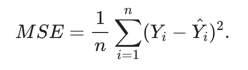
1. 평균 제곱 오차 Mean Square Error
2. 교차 엔트로피 Cross Entropy
두 확률분포 사이의 유사도가 클수록 작아지는 값이다. 모델을 학습하게 되면 ^y\hat{y}y^이 점점 정답에 가까워지게 된다.

읽을거리...
http://www.gisdeveloper.co.kr/?p=7631
손실함수(Loss Function) – GIS Developer
손실함수는 비용함수(Cost Function)라고도 합니다. 손실에는 그만큼의 비용이 발생한다는 개념에서 말입니다. 손실함수가 왜 필요한지부터 파악하기 위해 다음과 같은 데이터가 있다고 합시다. t =
www.gisdeveloper.co.kr
경사하강법 Gradient Descent
https://angeloyeo.github.io/2020/08/16/gradient_descent.html
경사하강법(gradient descent) - 공돌이의 수학정리노트
angeloyeo.github.io
learning rate 학습률
https://aileen93.tistory.com/71
[머신러닝] lec 7-1 : 학습 Learning rate, Overfitting, 그리고 일반화
#모두를 위한 립러닝 강좌 lec 7-1 : 학습 Learning rate, Overfitting 방지법, 그리고 일반화 https://www.youtube.com/watch?v=1jPjVoDV_uo&list=PLlMkM4tgfjnLSOjrEJN31gZATbcj_MpUm&index=18 *Gradient des..
aileen93.tistory.com
parameter 초기화
가중치 초기화 (Weight Initialization)
An Ed edition
reniew.github.io
오차역전파법 Backpropagation
MLP를 학습시키기 위한 알고리즘 중 하나. 출력층의 결과와 target 값과의 차이를 구한 뒤, 그 오차값을 각 레이어들을 지나며 역전파 하여 각 노드가 갖고 있는 변수들을 갱신해 나가는 방식이다.

전체 학습 사이클 수행
학습시킬 파라미터 초기화 코드
def init_params(input_size, hidden_size, output_size, weight_init_std=0.01):

    W1 = weight_init_std * np.random.randn(input_size, hidden_size)
    b1 = np.zeros(hidden_size)
    W2 = weight_init_std * np.random.randn(hidden_size, output_size)
    b2 = np.zeros(output_size)

    print(W1.shape)
    print(b1.shape)
    print(W2.shape)
    print(b2.shape)

    return W1, b1, W2, b2
학습시키는 코드(GPU 사용하지 않음)
# 하이퍼파라미터
iters_num = 50000  # 반복 횟수를 적절히 설정한다.
train_size = x_train.shape[0]
batch_size = 100   # 미니배치 크기
learning_rate = 0.1

train_loss_list = []
train_acc_list = []
test_acc_list = []

# 1에폭당 반복 수
iter_per_epoch = max(train_size / batch_size, 1)

W1, b1, W2, b2 = init_params(784, 50, 10)

for i in range(iters_num):
    # 미니배치 획득
    batch_mask = np.random.choice(train_size, batch_size)
    x_batch = x_train_reshaped[batch_mask]
    y_batch = y_train[batch_mask]

    W1, b1, W2, b2, Loss = train_step(x_batch, y_batch, W1, b1, W2, b2, learning_rate=0.1, verbose=False)

    # 학습 경과 기록
    train_loss_list.append(Loss)

    # 1에폭당 정확도 계산
    if i % iter_per_epoch == 0:
        print('Loss: ', Loss)
        train_acc = accuracy(W1, b1, W2, b2, x_train_reshaped, y_train)
        test_acc = accuracy(W1, b1, W2, b2, x_test_reshaped, y_test)
        train_acc_list.append(train_acc)
        test_acc_list.append(test_acc)
        print("train acc, test acc | " + str(train_acc) + ", " + str(test_acc))
Accuracy 확인
from matplotlib.pylab import rcParams
rcParams['figure.figsize'] = 12, 6

# Accuracy 그래프 그리기
markers = {'train': 'o', 'test': 's'}
x = np.arange(len(train_acc_list))
plt.plot(x, train_acc_list, label='train acc')
plt.plot(x, test_acc_list, label='test acc', linestyle='--')
plt.xlabel("epochs")
plt.ylabel("accuracy")
plt.ylim(0, 1.0)
plt.legend(loc='lower right')
plt.show()
Loss 확인
# Loss 그래프 그리기
x = np.arange(len(train_loss_list))
plt.plot(x, train_loss_list, label='train acc')
plt.xlabel("epochs")
plt.ylabel("Loss")
plt.ylim(0, 3.0)
plt.legend(loc='best')
plt.show()
'AIFFEL' 카테고리의 다른 글
| AIFFEL 아이펠 21일차 (1) | 2022.01.26 |
|---|---|
| AIFFEL 아이펠 20일차 (0) | 2022.01.25 |
| AIFFEL 아이펠 18일차 (0) | 2022.01.25 |
| AIFFEL 아이펠 17일차 (0) | 2022.01.25 |
| AIFFEL 아이펠 16일차 (0) | 2022.01.25 |


